Typically, no ferromagnetic materials are allowed in zone IV. With careful planning and approval, exceptions may be made to this rule.
Before all experiments, a plan document must be made and approved. Here is a template, and here is an example for the Lerner MR facility. You can edit the PDF to show your plan however you wish, as long as it is clear what you plan to do.
Once you have made the plan bring it to the safety officer for review. It must then be approved before every experiment by the study PI, and signed by two level II trained personnel after completion.
Some guidelines for a useful plan:
Number each object which will be moved into zone IV
Before moving anything, and after the time-out procedure, mark the locations in the room for each object with tape
Mark a tape line at a boundary lower than 5 Gauss field strength to never cross with magnetic material
Follow a specific order for bringing objects into the room
On completion, after removing the objects, remove the tape marking their locations to ensure you don’t forget anything
Save the signed and dated plan in your records and send a copy to the safety officer
Schedule a time on the google calendar at least 24 hours ahead to minimize interruption of clinical activity
If you are using a machine in a clinical area or have a human subject, dress professionally for patient/volunteer comfort
Find at least one other level II trained person to be in zone III whenever you are in zone IV, this can be a clinical technologist working at a nearby scanner
Insure a minimum of two level II trained personnel are present whenever a person is in zone IV, including at least one level II trained person in zone III
Gain prior approval from the study principal investigator for after hours scanning
Gain prior approval from the safety officer and/or study PI for all new devices or equipment to be used in zone IV
This project has two main elements: a Gadgetron-based reconstruction pipeline and a Unity-based visualization tool for the Microsoft Hololens 2. We’ll start by installing the application on the Hololens.
Hololens 2 Installation
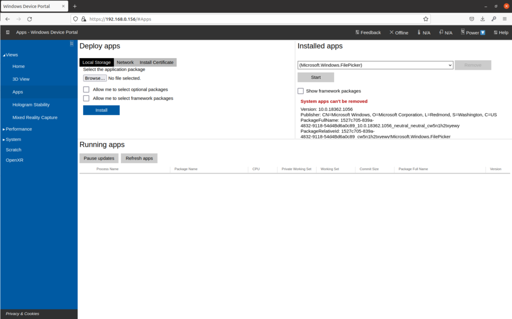
First, download the latest release of the Unity application from Github. You can also build the application from source if you so choose. Once you have downloaded and extracted the Unity release package, start by connecting to your Hololens 2 Device Portal through your computers browser. This will be hosted at the IP address of your device, but may require enabling developer mode in your settings. Navigate to the Views->Apps page. It should look something like this:
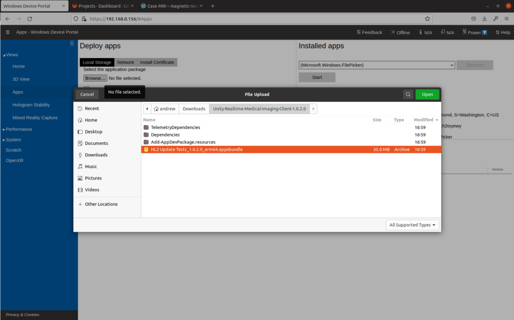
In order to install the application, click on “Local Storage” under Deploy Apps. Use the browse button to select the appxbundle inside the unzipped application folder:
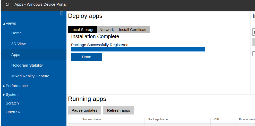
You can now click “Install” under the Deploy Apps section, and the installation will begin. You will eventually see “Package Registration Successful”, meaning the application is now installed:
Put on your Hololens 2 and open the “HL2 Update Tests” application from the Start menu. Once the application starts, you should see the below scene:
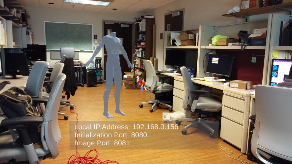
This is the “Initialization” screen of the application, meaning that it is waiting for a connection from the image reconstruction system. You can position the body as appropriate within this scene – wherever you place the body (and in whatever orientation) will determine the position and orientation of the visualized images once the system is running:
You are now ready to set up the Gadgetron reconstruction system to send images to your device.
Gadgetron Docker Configuration
While you can build and run the Gadgetron reconstruction pipeline from source, we encourage you to use the Docker container we’ve prepared as a starting point. If you need to install Docker, see this instructional guide.
Start by pulling the Gadgetron Realtime Cardiac docker image from the public Github Container Registry associated with this project’s repository:
Once the Docker image downloads, you are then able to start the reconstruction system using:
docker run -it -p 9002:9002 --gpus all ghcr.io/cwru-mri/gadgetron-cardiac-radial-grappa:latest
Breaking this down:
docker run || starts a docker container
-it || start the container interactively so we can see the logs in realtime
-p 9002:9002 || maps the Gadgetron port (9002) to the host machines port so that the system can be accessed outside of the container
–gpus all || allows the container to access the GPUs installed on your machine. (this project requires a CUDA-capable NVIDIA GPU)
ghcr.io/cwru-mri/gadgetron-cardiac-radial-grappa:latest || this is the image:tag pair that you are using as the source for your container
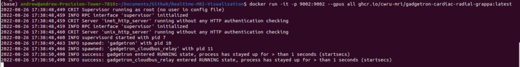
Once you run the above command, you will see the following status updates indicating that the Gadgetron and the supervisor daemons have successfully started:
You can now send data to the Gadgetron instance for reconstruction – however, the version of the Gadgetron ISMRM-RD client must match the version used within the Docker container. You can either install the appropriate version of Gadgetron and the necessary dependencies within a conda environment on your local machine, or simply use another instance of the same Docker image as your reconstruction runner.
Example Reconstruction
To test our system, we’ll be using a second copy of the same Docker image above, since this keeps version control a bit more simple (and is portable to any other machine too).
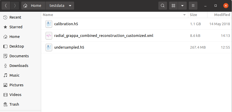
For the below exercise, I’ll be using the two datasets below as a test. Feel free to download them and follow along:
In order to use a Docker container as a reconstruction data client, we need to map the location of the source data into the container. For example, if my desired datasets were located at “/home/andrew/testdata”, we’d use the following command to start a container:
docker run -it -v /home/andrew/testdata:/tmp/testdata ghcr.io/cwru-mri/gadgetron-cardiac-radial-grappa:latest /bin/bash
Breaking down the new parts:
-v || maps a location on the local filesystem (/home/andrew/testdata) to a location within the new container (/tmp/testdata)
/bin/bash || by putting the bash command at the end of the docker run command, we can start a bash shell instead of another Gadgetron instance
Running the above (in a new terminal, not the one running your Gadgetron instance) and browsing to /tmp/testdata will show that this command successfully mapped our testdata folder into the container:
We can now use this client instance to start the image reconstruction process.
First, we need to run the “calibration” data and reconstruction pipeline in order to generate the necessary GRAPPA calibration files for the undersampled reconstruction pipeline:
gadgetron_ismrmrd_client -a 192.168.0.105 -p 9002 -f /tmp/testdata/calibration.h5 -c radial_grappa_combined_calibration.xml
Note that I’m including the IP address of my computer in the gadgetron_ismrmrd_client command to simulate the scenario where the Docker host isn’t your local machine. You can find your IP address by opening a new terminal and typing “ip address”. Look for the entry labeled “eth0” – your ip address should have the format xx.xx.xx.xx, followed by a subnet mask (“/24”).
With the weights generated, we can now run the undersampled data through its reconstruction pipeline (but don’t run this command yet):
gadgetron_ismrmrd_client -a 192.168.0.105 -p 9002 -f /tmp/testdata/undersampled.h5 -c radial_grappa_combined_reconstruction.xml
The reconstruction pipeline doesn’t know where to send the resulting data – we haven’t told it the IP address and port information of the Hololens 2 application we set up earlier. The easiest way to do so is by creating a copy of the “radial_grappa_combined_reconstruction.xml” pipeline configuration file and storing it next to your datasets. This way, you are able to directly edit the parameters of the pipeline, as well as the Hololens IP addresses, without needing to generate new Docker images. The file can be downloaded here – save it to the same testdata directory where our datasets are located, rename it to indicate it’s a customized version of the configuration file, then open it in a text editor:
I’ve isolated the section we care about in the block below. The bolded values below control the connection to the Hololens 2 device. As we saw during Hololens setup above, my device is available at a local IP of 192.168.0.156, with ports of 8080 and 8081, so I’ve filled in the appropriate values:
Once we make the necessary changes, we’ll be able to use the following command to run the reconstruction pipeline again, this time using our externally-provided configuration file (note the CAPITAL -C flag instead of lowercase this time):
gadgetron_ismrmrd_client -a 192.168.0.105 -p 9002 -f /tmp/testdata/undersampled.h5 -C /tmp/testdata/radial_grappa_reconstuction_customized.xml
Open up your Hololens 2 application, the run the above command. You should now see the reconstruction process run, and images should begin appearing:
You can manipulate, scale, window, and level the datasets using your hands as the controllers. Note that window/level controls are only applied as new data comes in – you can always hit run again on your reconstruction to see the data playback again.
If you want a single-line command for running the docker client reconstruction process, you can combine the commands above by replacing /bin/bash with the actual reconstruction client command as folllows:
docker run -it -v /home/andrew/testdata:/tmp/testdata \
ghcr.io/cwru-mri/gadgetron-cardiac-radial-grappa:latest \
gadgetron_ismrmrd_client \
-a 192.168.0.105 -p 9002 \
-f /tmp/testdata/undersampled.h5 \
-C /tmp/testdata/radial_grappa_reconstuction_customized.xml
Feel free to customize the source and target mount points as you see fit. You should now be able to take any of the Cardiac Radial Grappa source datasets and run them through the Gadgetron->Hololens visualization pipeline!
Instead of installing Matlab on your local machine, a better option is to run Matlab within a Docker container. This ensures that you are always starting with a clean environment, and allows you to very easily share your project in a reproducible manner.
The Basics
Running Matlab inside of Docker can be done with a single command:
docker run -it -p 8888:8888 --shm-size=512M mathworks/matlab:r2022a -browser
Breaking the command down:
run || starts a new docker container from an image
-it || interactive flag, means that the container’s execution will show up in the bash session you start the container from
-p 8888:8888 || port mapping, maps port 8888 inside the container to the same port on the computer you’re running the container on
mathworks/matlaScreenshot from 2022-08-24 12-38-21b:r2022a || the name/tag of the docker image to run
-browser || tells Matlab to run an interactive browser session for the GUI, hosted on http://localhost:8888/index.html
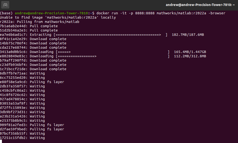
Once you run the above command, you’ll see the following:
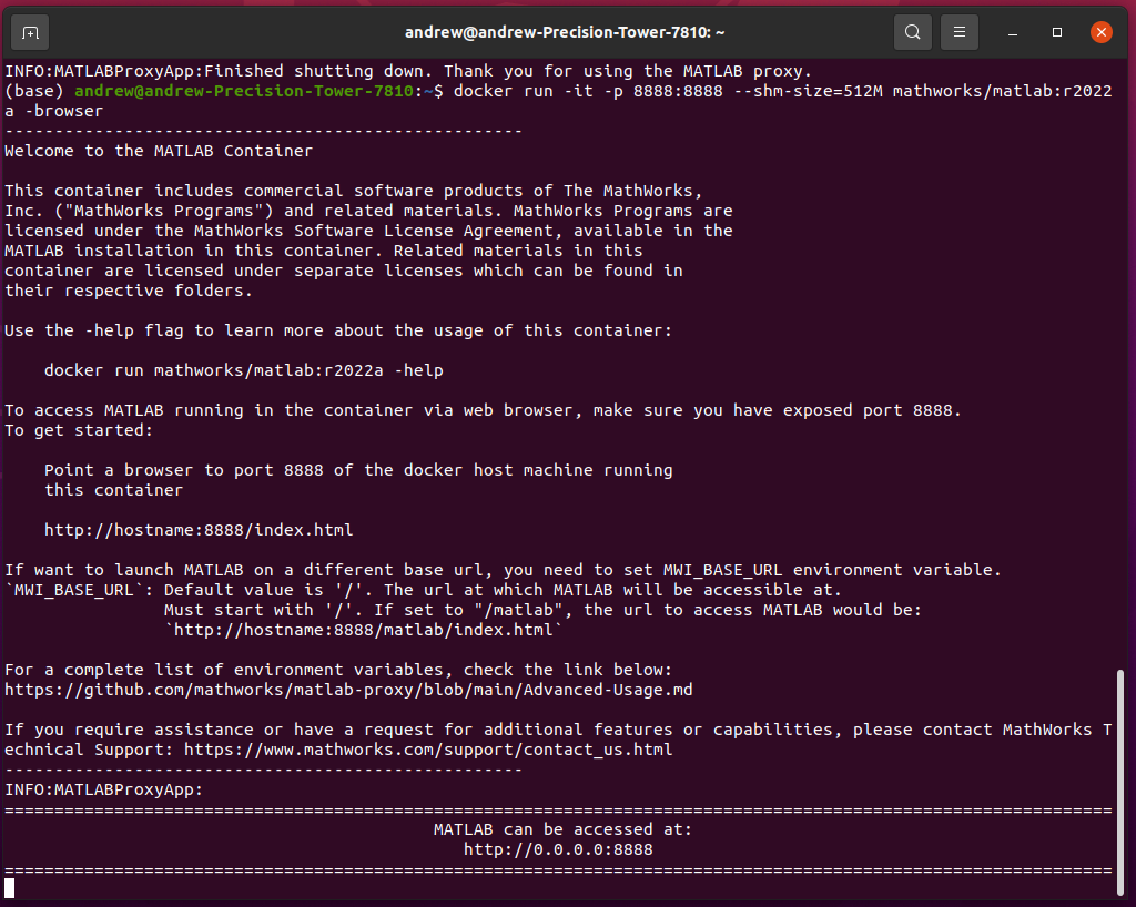
Your computer is now downloading the Matlab Docker image for r2022a. Once the download is finished, the container will start, and you’ll see the following:
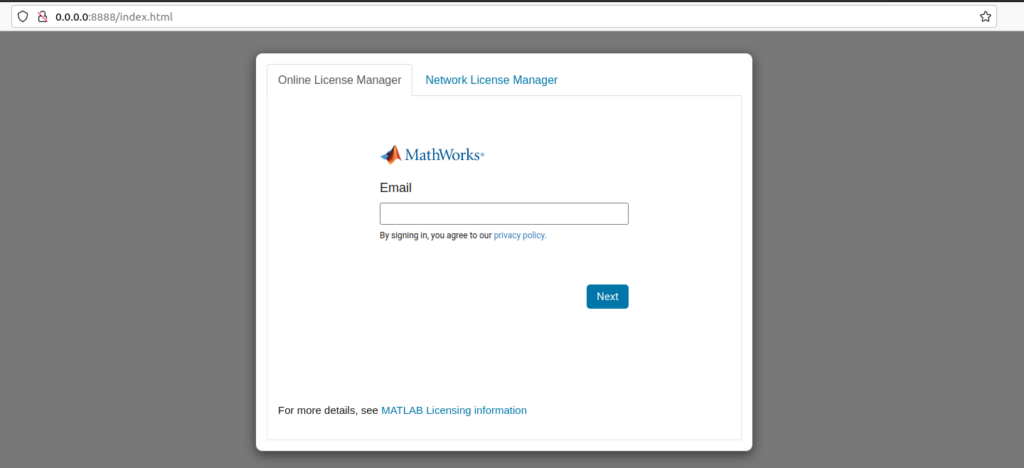
If you type the web address into your browser, you’ll then see:
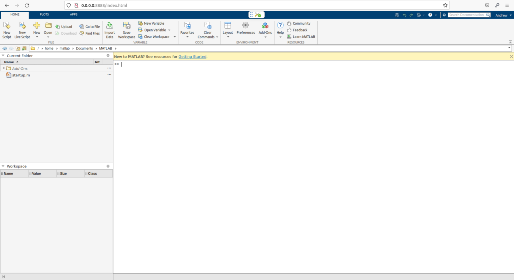
Log in to your CWRU Matlab account. Once you finish logging in, you should see a Matlab interface within your browser:
You are now running Matlab inside a clean Docker container. Note that anything you make/write inside this container is ONLY saved to the container (for now…. we’ll fix that later in this guide). But feel free to try using the Dockerized Matlab appliance now!
Changing Docker Images
The Docker image we used above (mathworks/matlab:r2022a) is a basic, clean installation of Matlab. However, for a lot of the work done in lab, we likely need some other toolboxes. Instead of using this as the base image, we can instead use Mathworks’ “Deep Learning” docker image as a base.
Doing so is as easy as changing the image in the run command to:
docker run -it -p 8888:8888 --shm-size=512M mathworks/matlab-deep-learning:r2022a -browser
Your computer will begin downloading the additional toolkit layers for the Docker image. Once it’s done, you’ll be all set to use the larger, more capable image instead.
Using GPUs
Now that we’ve changed to the Deep Learning image, we may also want to add support for the GPUs installed in many of our computers. Doing so is as easy as adding a flag to the run command:
docker run --gpus all -it -p 8888:8888 --shm-size=512M mathworks/matlab-deep-learning:r2022a -browser
This will forward the GPUs installed in your machine to the Docker container for use by Matlab.
Mounting Existing Code/Directories into Container
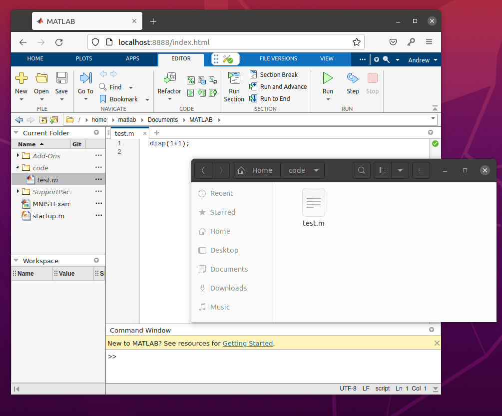
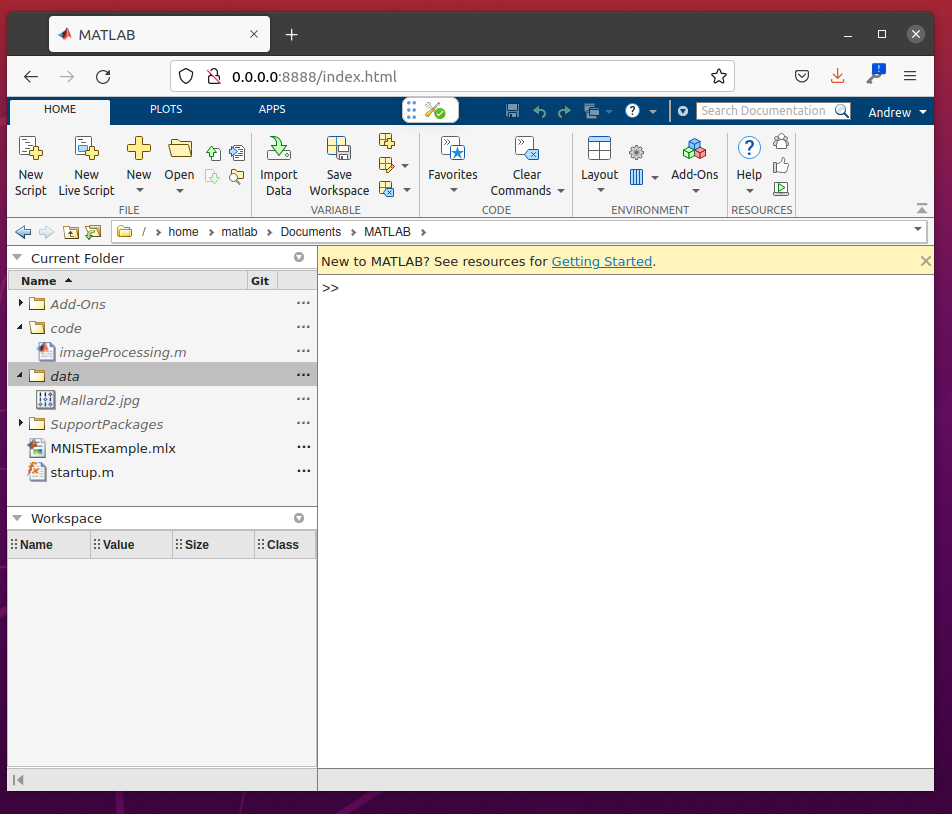
Most likely, you already have code that you’d like to open in Matlab. In order to do so, we need to mount the folder containing that code as a volume inside the Matlab container. In the below example, I’m mounting a directory called “code” that’s inside my user folder on the host machine to the default MATLAB directory inside the container:
As you can see, once Matlab starts up, the “code” folder and it’s contents from my local computer are now available within the running Matlab instance:
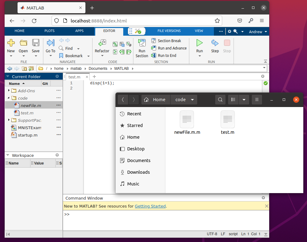
Just to test the functionality, try making a file inside the browser Matlab instance called “newFile.m”. You’ll see it show up in the local filesystem too:
Now, files you make will persist after you close the Matlab Docker container, as long as those changes are inside of a volume you have mapped to the container during startup.
Making and Sharing a Docker Image
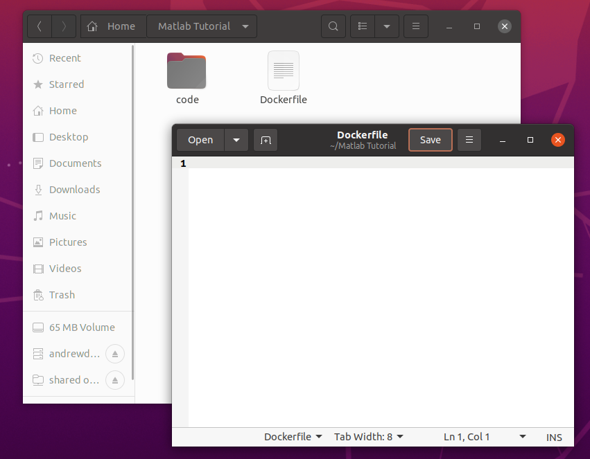
If you have a folder with some Matlab code inside it, this can also be used to quickly create a custom Matlab docker image that includes your code. We can do this with a very simple Dockerfile. Make a new, empty text file named “Dockerfile” in the directory above where your code lives:
Inside the Dockerfile, we’ll have three main lines:
FROM mathworks/matlab-deep-learning:r2022a
COPY code /home/matlab/Documents/MATLAB/code
CMD ["matlab"]
Breaking this down:
FROM || Specifies the source Docker image to use as the base for your new, custom image
COPY || Copies a folder or file from a location “code” to a location inside the new Docker image (/home/matlab/Documents/MATLAB/code)
CMD || Specifies the command to run when the Docker container first starts – in this case, Matlab
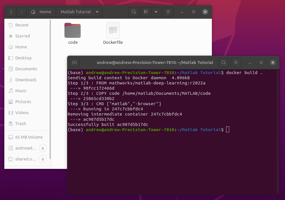
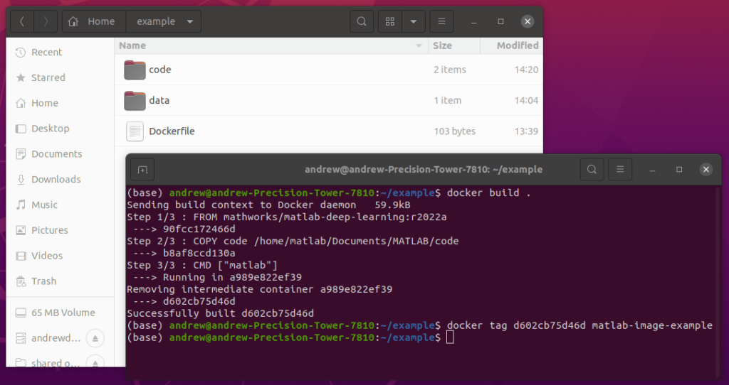
In order to build this new Docker image, we”ll open the root directory in the terminal and enter:
docker build .
Once the process completes, you’ll see:
You now have a custom Docker image containing your code, as well as a full installation of Matlab. To make things easier to keep track of, lets tag that new image with a human-readable name using:
docker tag ac987d5b17dc matlab-tutorial
You’ll need to replace the first part of the tag command with the hash given after the build process completed (after “Successfully built” in the screenshot above). Now that our new image is tagged, and we can easily run it with:
Once Matlab start up, you can see that our source code is included inside the image itself:
Importantly for the sake of reproducibility, the code inside this “built” version of the Docker container/image is now “read only”, unlike when you mounted the code folder as a volume. This means that anyone, anywhere who opens the Docker image you just built can run the exact same code you ran, and can’t edit it without making a copy inside the container. This is now a runnable, shareable, immutable version of your code.
If you want to see how to publish this Docker image to a Container Registry so others can use it, see this post.
The buildable sample we just put together can be downloaded below:
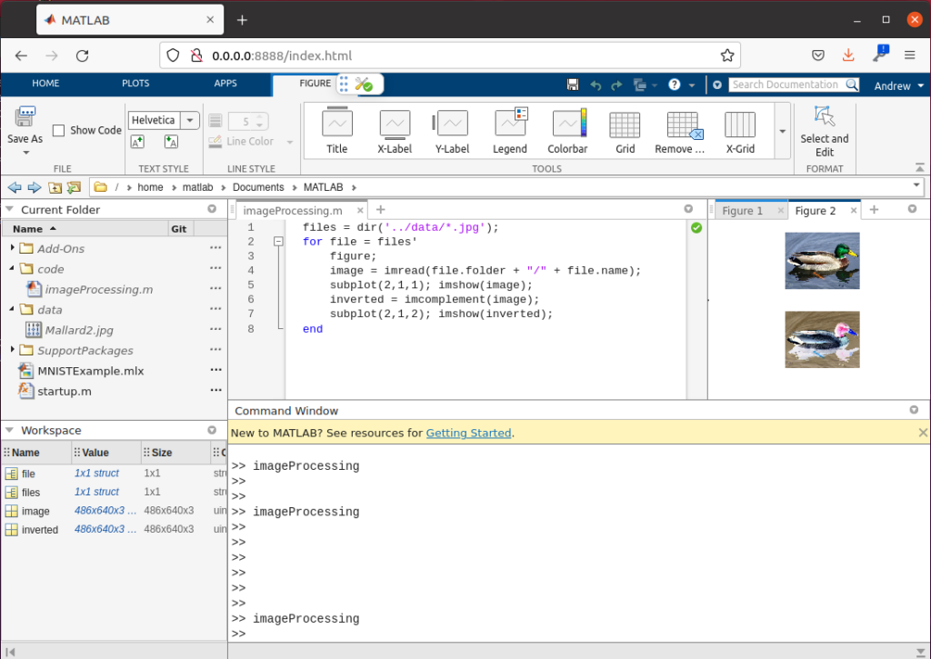
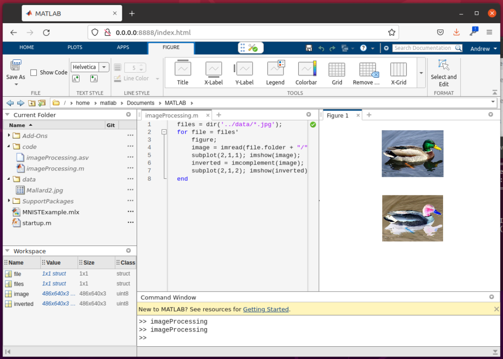
Lets image that we need to process a specific dataset, at a specific file location, with an existing set of Matlab code. In this case, we’ll start with some simple code that loads an image from file, displays it, inverts the colors, and displays the result as well.
We’ll start our development process by starting a docker container that maps a “code” location and a “data” location into the Matlab instance:
As you can see, both of the folders, as well as their contents, are now mapped into the running Matlab container:
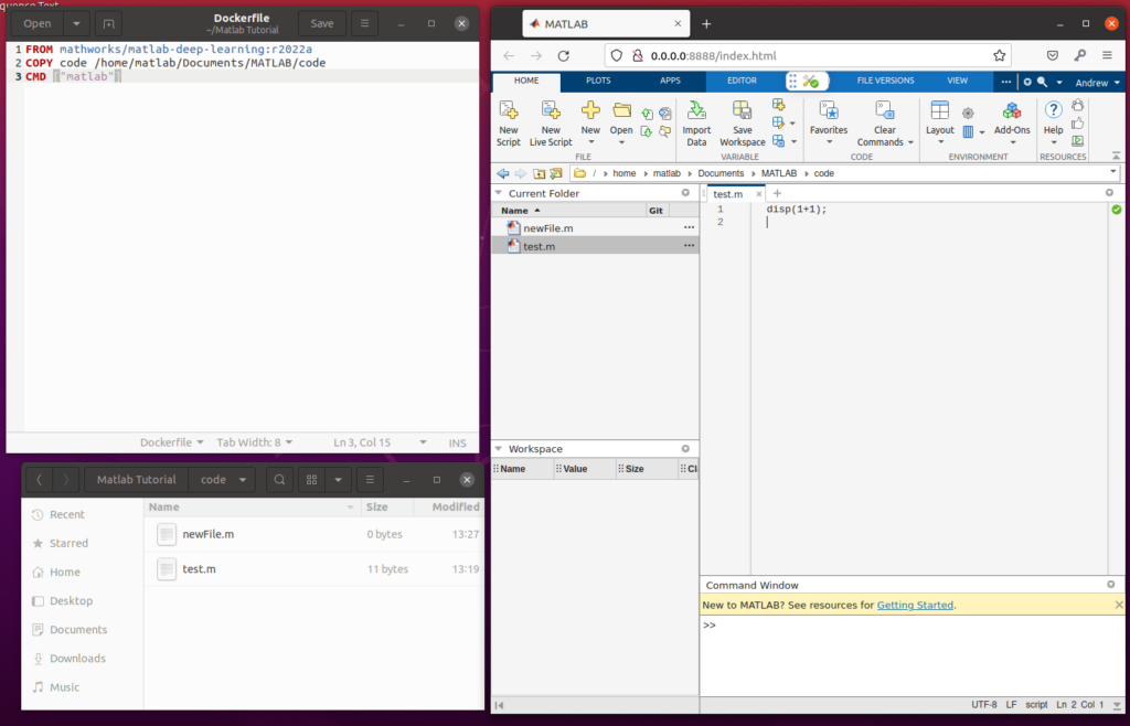
Now, we can start developing our data processing code. Anything we save while the code and data locations are mapped will be saved to the host machine as well. Here’s our basic code, and the results:
Now, lets build a docker container based on this project. We’ll use the same Dockerfile we wrote above:
FROM mathworks/matlab-deep-learning:r2022a
COPY code /home/matlab/Documents/MATLAB/code
CMD ["matlab"]
Notice that we’re not copying the “data” directory over to the Docker image, since there’s no reason to copy our datasets into the shared image. We’ll add this Dockerfile to the parent directory and run a build, then tag the result as matlab-image-example:
Now that the container is built, lets test it using the same dataset we used before. Since the data isn’t inside the container image (as we mentioned above), we’ll need to mount the data directory into the right location that we used in our code above:
docker run -v/home/andrew/example/data:/home/matlab/Documents/MATLAB/data -it -p 8888:8888 --shm-size=512M matlab-image-example -browser
As we can see, the Matlab instance that opened has the “code” in the proper code directory, as well as the same dataset inside of the data directory. However, the code is now “read-only”, as we can see from it being greyed out:
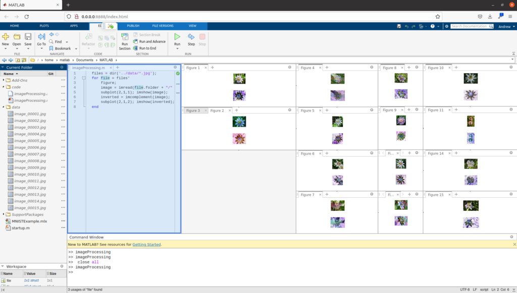
We now have a working data processing Matlab Docker container! Lets try testing with a different data set of 15 images that I downloaded from the web. Instead of moving this to the “data” folder we used for development, I can just start the Docker container directly, pointing to the folder in my downloads:
docker run -v /home/andrew/Downloads/flowers:/home/matlab/Documents/MATLAB/data -it -p 8888:8888 --shm-size=512M matlab-image-example -browser
Once Matlab opens, we’ll see that the new flowers dataset is mapped correctly into the data directory. Running the code now outputs 15 figures, one for each flower:
The source folders for the above example are included below:
You can continue extending this example with more mount folders (for example, a folder for results?), by allowing you to run the commands necessary from a batch terminal, and more. Additional documentation is available from Mathworks directly, for some of these more advanced use cases.